Calculate overlap reduction functions
Overlap reduction function calculation for arbitrary baselines
In this tutorial we will demonstrate how to calculate the overlap reduction function (ORF) for arbitrary baselines, which encodes the geometric sensitivity of a given detector pair as a function of the relative positions and orientations of the two interferometers.
First we import the necessary modules. We will use the Baseline module of pygwb. For more information on the Baseline module, we refer the user to the documentation page.
[8]:
import numpy as np
import matplotlib.pyplot as plt
import bilby
from copy import deepcopy
from pygwb.baseline import Baseline
import seaborn as sns
my_palette = sns.color_palette("colorblind")
Next we initialize empty Interferometer objects for LIGO Livingston, LIGO India, Virgo, Kagra, and Einstein Telescope. The latter is a TringularInterferometer object, which consists of three separate Interferometer objects at the vertices of an equilateral triangle. The Interferometer objects store the location information for each detector, like the latitude and longitude of the vertex and angle of the arms.
[2]:
L1 = bilby.gw.detector.get_empty_interferometer('L1')
A1 = bilby.gw.detector.get_empty_interferometer('A1')
V1 = bilby.gw.detector.get_empty_interferometer('V1')
K1 = bilby.gw.detector.get_empty_interferometer('K1')
ET = bilby.gw.detector.get_empty_interferometer('ET')
More information about the Interferometer object can be found here. For additional information on the bilby.gw.detector object, we refer the user to the documentation.
Next, we set the frequencies in each interferometer. We use a maximum frequency of 2048 Hz sampled with a spacing of \(\delta f = 1/T = 0.25~\mathrm{Hz}\), where \(T\) is the analysis segment duration:
[3]:
duration = 4
freqs = np.arange(0,2048,1./duration)
masks = []
for ifo in [L1, A1, V1, K1, ET]:
    if ifo.name=='ET':
        for i in range(3):
            ifo[i].strain_data.frequency_array = freqs
    else:
        ifo.strain_data.frequency_array = freqs
Now let’s define some baselines with the interferometers initialized above. This constitutes a pair of detectors. We define a few different baselines with the ET interferometers to demonstrate the ORF normalization for detectors with non-90-degree arms.
[4]:
L1V1 = Baseline('L-V', L1, V1, frequencies=freqs, duration=duration)
L1A1 = Baseline('L-A', A1, L1, frequencies=freqs, duration=duration)
V1K1 = Baseline('V-K', V1, K1, frequencies=freqs, duration=duration)
A1ET = Baseline('A-ET', A1, ET[0], frequencies=freqs, duration=duration)
ET01 = Baseline('ET 01', ET[0], ET[1], frequencies=freqs, duration=duration)
ET02 = Baseline('ET 02', ET[0], ET[2], frequencies=freqs, duration=duration)
ET00 = Baseline('ET 00', ET[0], ET[0], frequencies=freqs, duration=duration)
We need to tell the code for what polarization we are interested in calculating the overlap reduction function. For now, we assume that General Relativity is correct and look at the tensor polarization.
[12]:
fig = plt.figure(figsize=(12,8))
for ii,baseline in enumerate([L1V1, L1A1, V1K1, A1ET, ET00, ET01, ET02]):
    baseline.orf_polarization = 'tensor'
    if baseline.name == 'ET 02':
        ls='--'
    else:
        ls='-'
    plt.plot(freqs, baseline.overlap_reduction_function, label=baseline.name, ls=ls, lw=2.5, c=my_palette[ii])

plt.legend(loc='upper right', prop={'size':18})
plt.xlim(0,300)
plt.xticks(fontsize=18)
plt.yticks(fontsize=18)
plt.xlabel(r'$f~[\mathrm{Hz}]$', fontsize = 18)
plt.ylabel(r'$\gamma(f)$', fontsize = 18)
[12]:
Text(0, 0.5, '$\\gamma(f)$')
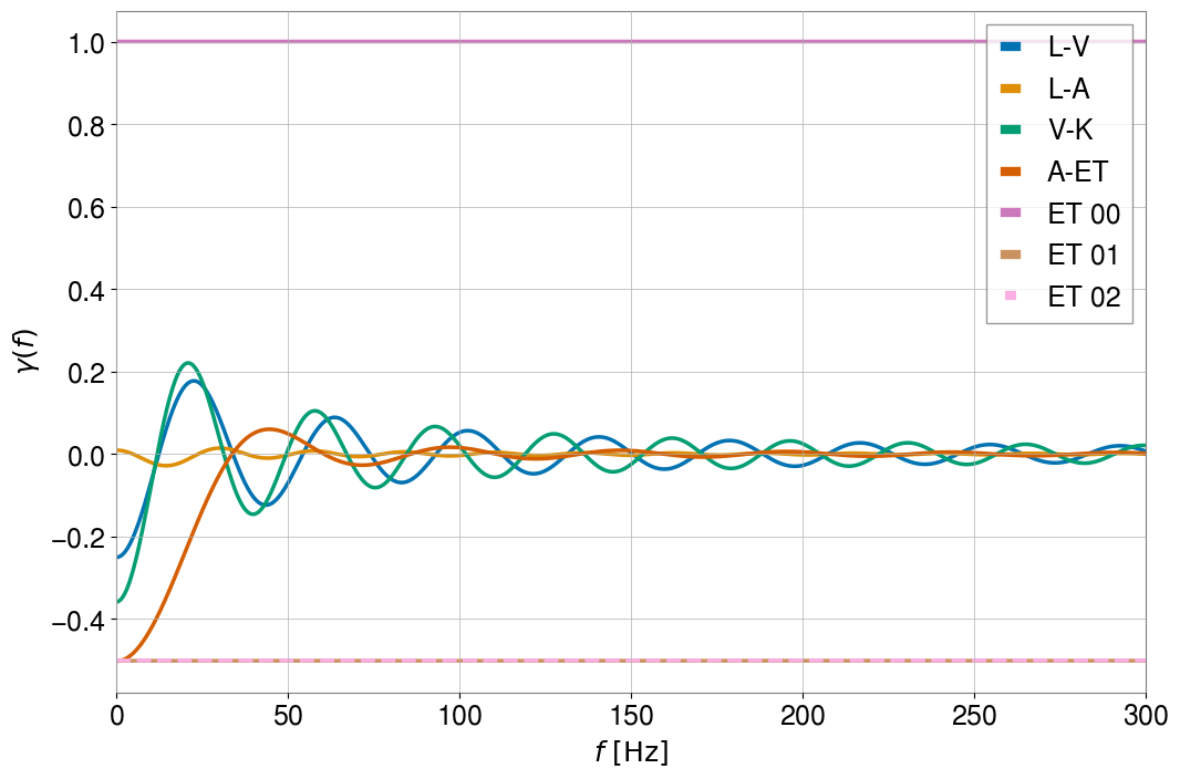
This plot shows us that the ORFs are normalized to be 1 for coincident and coaligned detectors irrespective of the opening angle between their arms. For additional information on the computation of the ORF, we refer the user to the documentation page of the module, as well as to the Baseline module to see how the two modules interact with one another.
Check normalization for ET
What about for coincident detectors that are rotated with respect to each other? This is the case for the ET01 and ET02 baselines, which are basically equivalent to two coincident ET detectors rotated by 120 degrees. Let’s verify this. First we make a copy of the ET[0] detector and rotate its x and y arm positions by 120 degrees. Then we create a baseline between the original ET[0] and this rotated copy.
[10]:
ET_rot120 = deepcopy(ET[0])
ET_rot120.xarm_azimuth += 120
ET_rot120.yarm_azimuth += 120
ET_test120 = Baseline('ET rot', ET[0], ET_rot120, frequencies=freqs, duration=duration)
ET_test120.orf_polarization = 'tensor'
Now we plot for comparison with the ET01 and ET02 baselines above.
[13]:
fig = plt.figure(figsize=(12,8))
for ii,baseline in enumerate([L1V1, L1A1, V1K1, A1ET, ET01, ET02, ET_test120]):
    if baseline.name == 'ET 02':
        ls='--'
    elif baseline.name == 'ET rot':
        ls=':'
    else:
        ls='-'
    plt.plot(freqs, baseline.overlap_reduction_function, label=baseline.name, ls=ls, lw=2.5, c=my_palette[ii])

plt.legend(loc='upper right', prop={'size':18})
plt.xlim(0,300)
plt.xticks(fontsize=18)
plt.yticks(fontsize=18)
plt.xlabel(r'$f~[\mathrm{Hz}]$',fontsize=18)
plt.ylabel(r'$\gamma(f)$',fontsize=18)
[13]:
Text(0, 0.5, '$\\gamma(f)$')
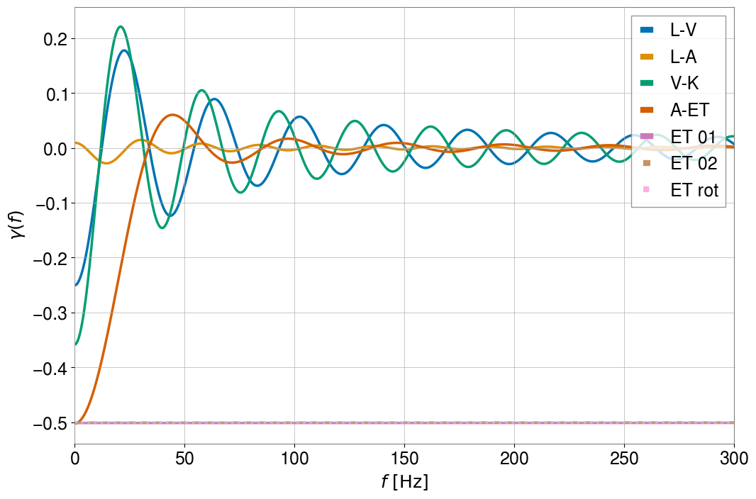
You can see that the three ET baselines lie nearly on top of each other, as expected. This tells us that the ORF normalization is such that \(\gamma(f=0) = \cos{\beta}\), for arm opening angles of \(\beta\).
Plot non-GR polarizations
In addition, the orfs module also allows non-GR polarizations. This is illustrated below for scalar polarizations, but it can also be calculated for vector polarizations.
[14]:
fig = plt.figure(figsize=(12,8))
for ii,baseline in enumerate([L1V1, L1A1, V1K1, A1ET, ET02]):
    baseline.orf_polarization = 'scalar'
    plt.plot(freqs, baseline.overlap_reduction_function, label=baseline.name, ls='-',lw=2.5, c=my_palette[ii])

plt.legend(loc='upper right', prop={'size':18})
plt.xlim(0,300)
plt.xticks(fontsize=18)
plt.yticks(fontsize=18)
plt.xlabel(r'$f~[\mathrm{Hz}]$',fontsize=18)
plt.ylabel(r'$\gamma(f)$',fontsize=18)
[14]:
Text(0, 0.5, '$\\gamma(f)$')

More information about how the ORFs are computed can be found in the documentation of the orfs module.